Relevance and regulatory requirements
Variable products are products whose cash flow structure cannot be derived deterministically, as there is no contractually agreed maturity and/or fixed interest rate. In practice, it is now customary to use mathematical models for this purpose.
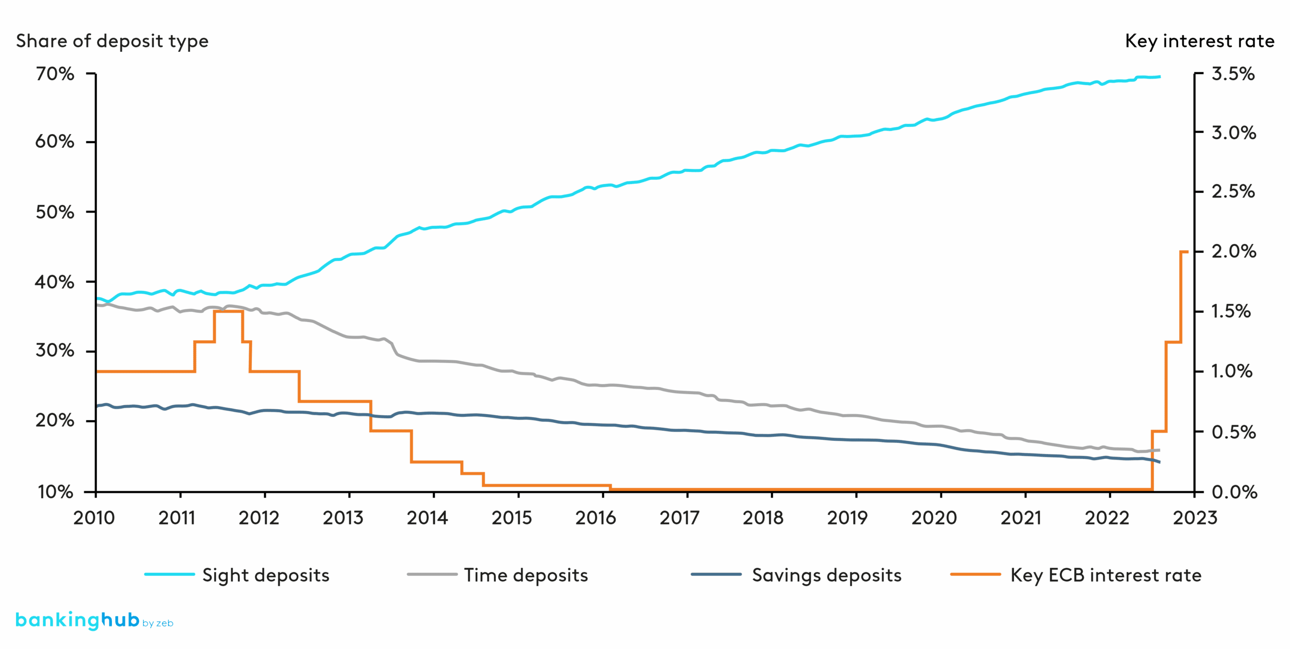
For an optimized bank steering and risk management, it is essential to use appropriate models in order to forecast reliable cash flow profiles. The increased importance of variable products with a stochastic cash flow profile can be explained, on the one hand, by new or further developed regulatory requirements (e.g. EBA IRRBB Guidelines[1], ECB ILAAP Guide[2]), but on the other hand also by the continuous and significant increase in volume of sight deposits as a typical variable product over the past ten years (see figure 1[3]).
In accordance with the requirements of MaRisk on liquidity risks[4] (BTR 3), institutions are required to prepare liquidity overviews by comparing cash inflows and outflows for the short, medium and long-term horizon. In this context, it is mandatory to consider both the normal and the stressed market conditions. This regulatory requirement implicitly mandates the modeling of cash flows.
According to Principle 3, Article 43 of the ECB ILAAP Guide[5], internal procedures and methods must be developed under the economic perspective to identify and quantify expected and unexpected liquidity outflows, as well as to incorporate the results when determining the internal liquidity buffer. According to Article 47, in order to ensure consistency, the assumptions made under the economic perspective should also be considered in the normative perspective, for example when calculating the forward LCR. Furthermore, they must also be used for stress test calculations and varied accordingly.
With regard to the choice of method for quantifying the risk of liquidity cash flows, neither MaRisk nor the ECB ILAAP Guide specify any explicit requirements. However, the ECB ILAAP Guide defines that the chosen procedures and assumptions “are expected to be robust, sufficiently stable, risk-sensitive and conservative enough to quantify liquidity outflows that occur rarely” (Article 72). There is an additional requirement that these methods be fully understood and appropriate to the institution’s situation and risk profile (Article 75).
Due to the market developments and regulatory requirements described above, it is becoming increasingly important that institutions reliably and accurately determine the maturities of their portfolios. Non-quantitative estimates of cash flow maturity forecasts based on experience and expert knowledge, as carried out in the past and even today, are regarded as inaccurate and not reproducible. Also, zeb’s experience from projects and audit findings has found them to be inadequate. The supervisory authorities expect well-founded, quantitative models.
Comparison of approaches to modeling liquidity cash flows
Below, we will present different quantitative approaches and methods for modeling liquidity cash flows and discuss their respective advantages and disadvantages. There are many other methods that can be used in cash flow modeling (e.g. Monte Carlo simulations), which, however, will not be addressed in this article. In our opinion, the methods described below are superior to the other methods in terms of their cost-benefit ratio.
Parametric methods for liquidity modeling
Parametric methods, in particular, are widely used in the context of quantitative modeling of future liquidity cash flows. These assume the same fluctuations behavior of the cashflows at two different points in time and carry out an approximation based on historical data. Typical distribution models applied in this context are, for example, a standard normal distribution or a log-normal distribution.
Since a constant distribution over time is assumed, the results of parametric methods do not take into account trends and seasonal components. If required, however, they can also be combined with a regression model (e.g. linear, exponential, sine/cosine).
Despite the undifferentiated approximation of all liquidity cash flows, e.g. by a standard normal distribution, in our opinion this method represents a significant improvement and is a useful extension to a non-quantitative estimation, as the quantitative results are reproducible and comprehensible. Furthermore, due to their low complexity, parametric methods are fairly resource-efficient and provide reliable results even when based on a limited amount of data. They can thus be set up and operated with little effort.
Advanced time series models (e.g. ARIMA-based)
To model liquidity cash flows even more accurately, we can use more complex methods with more parameterization flexibility. These methods, however, require a high-quality and fine-grained data set in order to achieve a significant advantage over simple parametric methods. Furthermore, the additional effort has to be weighed against the increased benefit to ensure that it is in proportion.
If, however, these conditions are met, the use of advanced time series models should certainly be considered. Especially ARIMA-based methods are gaining ever more relevance and attention in the context of liquidity cash flow modeling. These methods forecast time series under the assumption that each value at a certain time t is dependent on the values of the time series before t. The model can thus be approximated with the help of historical time series and forecast on that basis.
There are numerous extensions to the ARIMA model. One of these is the ARIMAX model, which adds exogenous variables to parameterize an external trend. While trends are also represented by the ARIMA model, this is limited to those that are also intrinsically present in the historical time series. As mentioned above, however, the volume of sight deposits is determined by external factors (e.g. interest rate rises, inflation). Since external influences change the general conditions over time, such trends can only be represented by using exogenous variables.
Another extension is the so-called SARIMA model, which approximates an additional seasonal pattern of the time series. Sight deposits normally have periodic patterns with a monthly frequency, which can be reproduced excellently by the SARIMA model. The extended SARIMAX model even takes into account both exogenous trends and seasonal patterns.
While the model parameters can be estimated objectively by least squares and maximum likelihood methods, the correct choice of specification parameters is of high importance for a reliable prediction of the time series and represents the greatest challenge in cash flow modeling. Similarly, the decision whether to use an ARIMA, ARIMAX, SARIMA or SARIMAX model is not always trivial. The SARIMAX model does not necessarily provide a more reliable forecast than the ARIMA model, and it requires intensive reconciliation effort with respect to the available data.
It is possible to perform a best-fit comparison with the historical data for various specification parameters and thus determine the statistically best choice for the available data in a largely automated manner and with little effort. With this approach, it is possible to work with very few subjectively made assumptions.
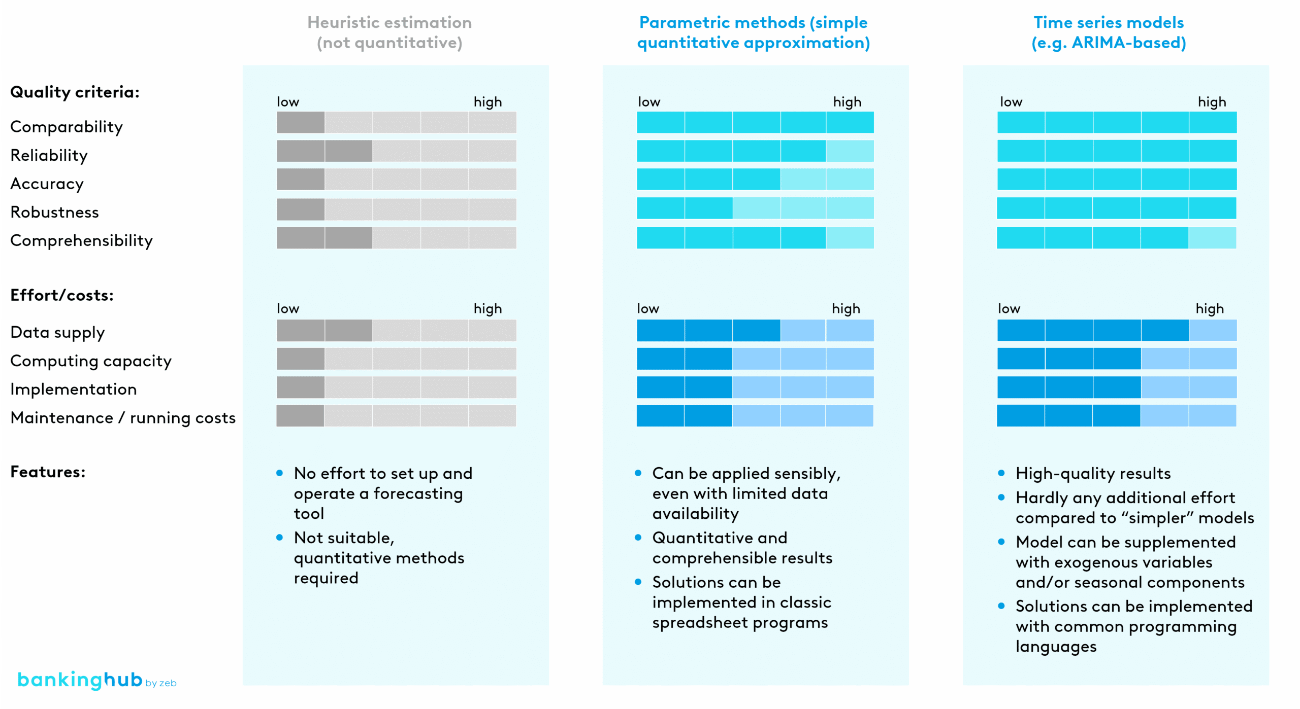
A comparison with the simple parametric methods shows that ARIMA-based methods can achieve significantly more accurate results in forecasting. The advantages are particularly evident when data sets are available at short intervals (preferably daily) over a long period of time.
Artificial intelligence (brief outlook)
Another method conceivable for forecasting liquidity cash flows is to use a model generated by machine learning. At present, artificial intelligence (AI) is a rapidly evolving topic area whose application is being tested and examined across a wide variety of domains (see, for example, our BankingHub article “LCR forecasting with AI”[6]).
Compared to the modeling approaches described above, this method offers the distinct advantage that the AI model can be trained with any other data in addition to the standard historical data. This makes it possible to consider further influencing factors (e.g. customer characteristics or current market data) for the forecast of liquidity cash flows.
The biggest challenges in implementation, however, are usually insufficient data and a lack of transparency of the model results (“black box” algorithms). AI models therefore only partially meet the regulatory requirement for traceability of the methods used, and it may prove difficult to interpret the results.
Challenges in implementation
In addition to the methodological challenges described above, an implementation also involves many practical hurdles. One of them is the required database: especially at the product level, a sufficient amount of historical data is often non-existent or only available on a monthly basis, meaning that the samples are too small for reliable forecasts. If, on the other hand, long time series are available, their representativeness should be critically questioned.
Seasonal occurrences, such as a credited thirteenth salary, should also be represented if they are considered material. Further exogenous factors, such as the interest rate level, GDP, inflation, etc., should be taken into account depending on their determined significance. This proves once again, that a good database is required for the corresponding statistical tests.
It is also important to select the most suitable portfolio segments to model the specifics of the various products and customer segments. On the other hand, it is also necessary to maintain a materiality threshold, and individual customers should not be able to shape the behavior of a portfolio, as this makes statistical cash flow modeling impossible. Especially in wholesale banking, it may prove advisable to model the liquidity risk of very large transactions separately.
In accordance with the proportionality principle, the dimension of the selected model should be based on the business model and the complexity of the respective institution. It may well be advantageous to give priority to a simpler approach over a very complex model if a good forecasting quality can still be achieved.
From both a business and supervisory perspective, it is necessary to interpret the results in order to incorporate them meaningfully into bank management. To this end, a cash flow model must also adequately take into account new developments such as interest rate portals and comparison sites, which may well lead to lower customer loyalty in the future.
It is also important to apply cash flow modeling approaches consistently across divisions in order to avoid conflicting management impulses. As an example, it is particularly important to ensure the consistency and reconcilability of the cash flow modeling assumptions and cash flows used in risk controlling and FTP (funds transfer pricing).
Modeling approaches must be evaluated according to institution-specific circumstances
We have compared different quantitative approaches to modeling liquidity cash flows for variable products and conclude that there is no universally optimal solution. The effort and benefits of the respective approaches must be weighed up individually for each institution.
The provision of high-quality data notably poses challenges for some institutions. If such a database is not available, even a very advanced time series model will not be able to provide significantly more accurate results, and it is advisable to resort to simpler parametric methods in this case. If, however, an institution requires more accurate forecasts, including non-stationary structures such as seasonalities or exogenous factors, they can resort to more advanced methods such as the ARIMA-based methods, provided that a high-quality database is available.